Is Tetris Biased?

My first experience with stochastic processes was in 1989, with Tetris on the Nintendo Gameboy. Each of the seven Tetris pieces arrived one at a time, chosen by some mysterious intelligence who seemed to know exactly which pieces I didn’t want. In the early 1990s, I had no way to tell how this process worked, or confirm whether it really was biased in some way, but with modern tools - primarily the R programming language - and plenty of free resources online, this is a straightforwards exercise.

The first thing to know about the Tetris randomizer is there is no one randomizer, as it has changed in almost every edition since Alexey Pajitnov’s original uniform sampler in 1984.¹ To Tetris aficionados, two key phenomena determine the quality of a particular randomizer: droughts, which are the periods before a piece reappears, and floods, in which a piece appears multiple times in a row. Since 2001, official copies of Tetris use the “7-bag” randomizer, in which the seven pieces are output in randomly ordered sets. The two algorithms I will focus on here are the ones I grew up with, for Tetris on the NES and the Gameboy, both released in 1989.

Two 1989 Algorithms

As a pair, the 1989 NES and Gameboy versions of Tetris have sold 43 million copies, making them some of the most popular games ever.² Both versions were written in Assembly, using the instruction set for the NES’s MOS 6502 processor and for the Gameboy’s Sharp LR35902. By looking at this hexadecimal machine code, hobbyists have reverse-engineered each algorithm, and from their descriptions we can see the two algorithms work quite differently.

The NES algorithm samples one piece randomly and compares it against the last piece in the sequence. If the two are the same, it draws a second piece as replacement (which may also be a repeat).³ In contrast, the Gameboy algorithm takes the last two pieces into account, combining them through a bitwise OR operation with the candidate piece. If the candidate is too similar to this combination, the algorithm samples another candidate and checks again. If that is too similar, it samples a third time and returns it that no matter what.⁴

Although both were released in 1989 by Nintendo, the Gameboy algorithm was written first⁵, followed by a rewrite for the NES a few months later. Why the NES uses a new algorithm is unclear, but the answer may lie in how each algorithm behaves over many, many draws.

Using R for Simulation

It’s prohibitively difficult to describe each algorithm in the “real world” of Tetris gameplay, since it takes a long time to observe even a few hundred draws. We can instead write stochastic simulations of each, and draw from these as many times as we like. In the programming language R, I’ve written a package called tetristools and its core function, rtetris.⁶ Like most random number functions in R, e.g. rnorm, runif, etc.), we tell rtetris how big of a sample we want, and it generates pieces as character vectors⁷.

library(tetristools)
x_gb <- rtetris(1e7, algo = "gameboy")
x_nes <- rtetris(1e7, algo = "nes")

par(mfrow = c(1, 2))
barplot(table(x_gb), border = NA, col = "dodgerblue", main = "Gameboy",
    yaxt = "n", ylim = c(0, 15e5))
abline(h = 1e7/7, lty = 2)
axis(2, at = c(0, 5e5, 10e5, 15e5))
barplot(table(x_nes), border = NA, col = "dodgerblue", main = "NES",
    yaxt = "n", ylim = c(0, 15e5))
abline(h = 1e7/7, lty = 2)
axis(2, at = c(0, 5e5, 10e5, 15e5))

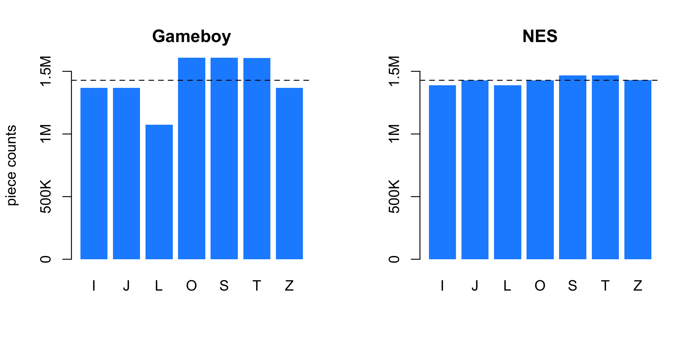
Simulating ten million draws from each, we can see right away that something is wrong with the Gameboy algorithm. Several hundred thousand L pieces are missing, there are far too many O, S and T pieces, and a clear bias against J, Z and I. With so much data, we can think of these counts as a limiting probability distribution of outcomes, e.g.

round(100 * (prop.table(table(x_gb))), 1)
> x_gb
>    I    J    L    O    S    T    Z 
> 13.7 13.6 10.7 16.1 16.0 16.1 13.8 

round(100 * (prop.table(table(x_nes))), 1)
> x_nes
>    I    J    L    O    S    T    Z 
> 13.9 14.3 13.9 14.2 14.7 14.6 14.3

In comparison to a 14.3% chance under uniform sampling of seven options, the Gameboy has a cumulative bias of over five percentage points towards O, S and T, and penalty of about -3.5% against L. In comparison, the NES algorithm favors S and T, and also disfavors I and L, but none of the NES biases are greater than half a percentage point.

Markov and Tetris

The tabulated counts are enough to identify some strange pathologies, especially in the Gameboy randomizer, but we can do much, much better. The description of the NES randomizer implies that the choice of next piece is dependent on the current piece, that is, the NES algorithm is a first-order Markov process. As such, we should describe the seven conditional probability distributions for each of the seven “states” the system could be, in based on the seven pieces. Expressed as percentages:

current_piece <- x_nes[1:(length(x_nes) - 1)]
next_piece <- x_nes[2:length(x_nes)]
round(100 * (t(apply(table(current_piece, next_piece), 1, simplex))), 1)
>             next_piece
>current_piece    I    J    L    O    S    T    Z
>            I  3.2 15.5 15.6 15.6 19.0 15.5 15.6
>            J 15.6  3.0 15.5 15.6 15.7 18.7 15.8
>            L 15.6 15.7  3.2 15.7 15.6 18.6 15.7
>            O 15.7 15.6 15.8  6.1 15.7 15.7 15.5
>            S 15.6 15.7 15.7 15.7  6.3 15.6 15.5
>            T 15.6 15.7 15.7 15.6 15.6  3.1 18.7
>            Z 15.8 18.7 15.7 15.5 15.5 15.7  3.2

Unlike the barplot above, this Markovian transition matrix completely describes the NES algorithm, with each row representing a state-dependent probability distribution. If we wished, we could perfectly replicate the NES’s behavior by sampling recursively from this, with each choice determining the next row to use. So written, we can see that the algorithm is heavily biased against two-in-a-row sequences, but also has a few odd biases not visible from the piece frequencies:

• I favors S
• J & L favor T
• T favors Z
• Z favors J

This is one of the great paradoxes of conditional versus marginal probabilities: none of the seven states bias against the all-important I piece, but in the aggregate there is a bias.⁸

We could make a similar table for Gameboy draws, but that would be inaccurate because the algorithm depends on both the current piece and the last piece in the chain. It is a second-order Markov process, and we must define 49 states from the 7 $\times$ 7 possible combinations of the last two draws, and describe a conditional probability distribution for each one. Or, to look at it another way, we need seven different transition matrices to fully describe the system:

last_piece <- x_gb[1:(length(x_gb) - 2)]
current_piece <- x_gb[2:(length(x_gb) - 1)]
current_state <- paste0(last_piece, current_piece)
next_piece <- x_gb[3:length(x_gb)]
round(100 * t(apply(table(current_state, next_piece), 1, simplex)), 0)
>             next_piece
>current_state  I  J  L  O  S  T  Z
>           II  1 20  1 20 19 20 19
>           IJ 14 14 14 15 14 15 14
>           IL  1 20  1 20 19 19 19
>           IO 14 15 14 14 14 14 15
>           IS 14 14 14 14 14 14 14
>           IT 15 14 14 15 14 14 14
>           IZ 14 14 14 14 14 15 14
>           JI 15 14 14 14 14 14 14
>           JJ 19  1  1 19 20 20 20
>           JL 20  1  1 19 20 20 19
>           JO 14 14 15 14 15 14 14
>           JS 14 14 15 14 15 14 14
>           JT 14 14 14 14 15 15 14
>           JZ 14 14 14 15 15 14 14
>           LI 14 14 14 14 14 14 14
>           LJ 15 14 14 15 14 14 15
>           LL 17 16  0 17 17 16 16
>           LO 14 14 14 14 15 14 14
>           LS 14 14 14 15 14 14 14
>           LT 14 14 14 14 14 14 15
>           LZ 14 14 15 14 14 14 15
>           OI  5  5  5  5 27 27 27
>           OJ  5  5  5  5 27 27 27
>           OL  4  4  5  5 27 27 27
>           OO  4  5  5  5 27 27 27
>           OS 14 14 15 14 15 14 14
>           OT 14 14 14 14 14 14 14
>           OZ 14 14 15 14 14 14 14
>           SI 14 14 14 15 15 14 14
>           SJ 27  5  5 27  5 28  5
>           SL 28  5  5 27  4 27  5
>           SO 14 14 15 14 14 14 14
>           SS 27  5  5 27  5 27  5
>           ST 14 14 14 14 14 14 14
>           SZ 27  5  5 27  5 27  4
>           TI  5 27  5 27 27  5  5
>           TJ 15 14 15 14 14 14 14
>           TL  5 27  4 27 27  5  5
>           TO 14 14 14 15 15 14 14
>           TS 14 14 15 14 14 14 14
>           TT  5 27  5 27 27  5  5
>           TZ  5 27  4 27 27  5  4
>           ZI 14 14 14 14 14 14 15
>           ZJ 14 14 14 14 14 14 14
>           ZL 20 19  1 19 19 20  1
>           ZO 14 14 14 15 14 14 14
>           ZS 14 14 14 14 14 14 14
>           ZT 14 15 14 14 14 14 14
>           ZZ 19 19  1 20 19 20  1

From this, we can see some very large biases in the Gameboy algorithm, with some pieces being penalized below 1% (an I after I, L), and others being greatly favored (an O after two T’s).

Both the NES and Gameboy transition matrices also imply the existence of modal loops that are more likely to occur than any others. For the NES, it is J $\rightarrow$ T $\rightarrow$ Z $\rightarrow$ J, though the biases here are small. For the Gameboy, the O, S, and T pieces become highly biased towards each other if another piece is in-between, and this ‘citation ring’ leads to their over-representation in the Gameboy’s marginal distribution.

Predicting Drought Lengths

A critical calculation is the period of time between two “I” pieces, called a drought. With the modern 7-bag randomizer, this cannot last longer than 12 pieces, but since both NES and Gameboy’s algorithms are probabilistic, there is no upper limit on how long a drought can last. Taking the simulations above, we calculate the drought lengths between I pieces as:

hits <- which(x_gb == "I")
drought_lengths <- diff(hits) - 1 # t
drought_pmf <- prop.table(table(drought_lengths)) # pr(X = t)
drought_cdf <- cumsum(drought_pmf) # pr(X <= t)
drought_ccdf <- 1 - drought_cdf # pr(X > t)

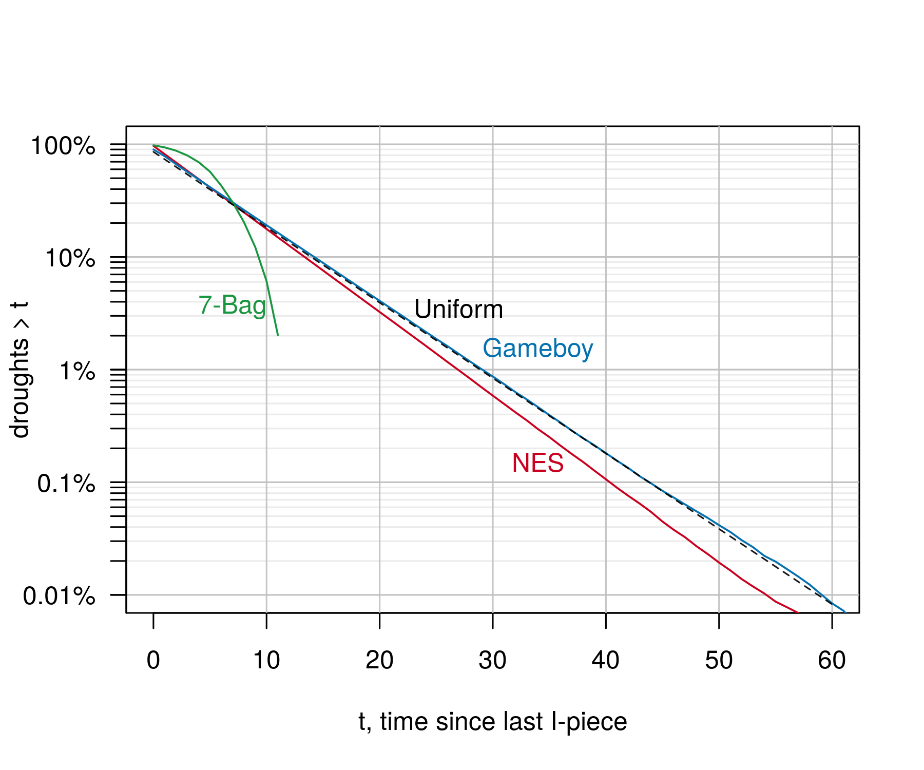
The average drought length for the NES is 6.2 pieces, and for the Gameboy, 6.3, but with an exponential decay this not especially useful to know. Graphing the cumulative probability the drought lasts as long as any length $t$ implies that the drought duration follows a power law for both NES and Gameboy, with the NES having a slightly faster decay rate. For example, a drought longer than 20 pieces will occur 3.3% of the time on the NES, and 4% of the time on the Gameboy, and a drought longer than 40 occurs twice as often on the Gameboy (0.2% vs 0.1%).

It’s useful to compare both of these against what you would expect under purely random draws, where droughts would follow the Geometric distribution. Using R’s built-in Geometric probability functions, 1 - pgeom(20, 1/7) is 3.9% (dotted line), which closely tracks with the Gameboy.

Conclusions, and a Problem

Simulating out chains of draws from each algorithm and playing around with them in R has answered our question. Compared to simple random sampling, both the NES and Gameboy randomizers do a good job at flood prevention - the Gameboy’s second-order transition matrix highly penalizes all three-in-a-row outcomes, and the NES’s first-order matrix penalizes two-in-a-row outcomes. However, we’ve also identified severe biases with the Gameboy algorithm, which probably explains why it was quietly replaced in late 1989 for the NES release. Even on the official NES release, though, Tetris has some small but detectable biases. As an exercise in learning new things about a game dear to many, the simulation approach is satisfying.

But there’s also a big problem with the above analysis (or any such analysis) - how do we know if our simulation is accurate to the “real world” of Tetris games? The reverse-engineering of the code may be flawed, or my implementation in tetristools. To really be sure, we must treat the above as predictions, and compare them against actual Tetris game data using statistical modeling, which we will take on next time.