In my last post, I simulated millions draws from two versions of the piece randomizer inside Tetris. The 1989 algorithm for NES Tetris can be described as a first-order Markov process, biased against repeat pieces, while the Gameboy algorithm is a more complex, second-order process with some seriously strange biases. At least, that’s what the simulation says. Here we use real Tetris data to find out if these simulation models are accurate, using the Stan language to fit simple multistate Markov models.

The Data

My daughters and I recorded several hundred real Tetris sequences, from both the official 1989 NES edition and the 1989 Gameboy edition.¹ After three rounds, we had these 579 draws from the NES:

ZJLTSJTZJILJISJOTLTTJTISZOZSLTIJTZIZSSJSLZSLJTIOIOIJLOSOLJLOTZTIZSJIZSZJOLOZTSZJOJOTTOLOJSTOLTOSTILZISTLZLZITJIOJOTJLOTLOTOILJTZOTLSJZLOSTJSZLTOTLLZLOZOSTITSLOLIOSOOTOTIZTZOLISOTJIOLSOLZJLZTJOITJZZTISSLSJTISTSISZJJOSOLZTLOSLJIZOSLTL|SSIOZLTISISIOLIJSLZIJISSIZSLTSSILTJZSOZIOTOZOISTJILIJIZLJTJOLJZOIZOIOSOZSLSZJJIOJZTLTSJOSTTOTIOTLJLSOTSLSOOZIJOJOTOTLZJLZTOZITILISTILZZJSTJIJTSTSOZSLOIIOJISLZLIJOLOSZISOSO|ITOSTISSLISISZOILOOJLJSJZOZILTJZTIZOISOJSJZZIJIZLIZSOLZIJSIZOJOJSILJOLTZISLZIOOZLIZTIJLIZSOSSZIZTJIJZSJZJSZOTZOIJZZZTIZSIJILITLILZOZTJSOJZTZSIIIOJOJJLTZLTZTIOILZZTSITZTJLSJZTIL

Each of the seven Tetris pieces is represented by a letter, with the three rounds separated by “|”. We also played four rounds on the Gameboy, with 692 draws as follows:

SOITISIITZSOTJSSTTSJZOJZOJTJLZJZZOOSOTTOTZOZTLSJOLSSOTSJILTJLSTIOJSLTLJSSSOZSJTIOISSOJJSLOTOLSOZZSIJOOSLOJSOOZOTLOTJSLTZSJTOSSSO|ITLOTSTLISTJSIJOZISOZLTJSSLOJTLSZ|SIOJZZOISZOOZTTJLTISLISILTTJSZOOTOJTOSJIOTLSJTISJZJTZOLSZOJTOJTOJOJSZTIJZOJZSTLOLTLOSTLJJIOSZJZJITSOSJISZ|IJJSIOOZSLOTTJTIJTOISJOIOLZSTSJTSOJJOOZJSLLJOSISOLTIOSJOJJOIOZZTTJLIZOOSSIJITJOSOITLJJZSTIJSOIZJIOSJTIJTSTTTJLTLIJLIITLOIITLJTLOZSLTLSOOSSSZTSOIZLIZLTL|TJSJOLTIJOLZIOJZOLZLOSZTLJIZZIITTOSIOOSZTIOITZJISOOJZTJILJJZLLTISJJZTIOJZLLTSOJZOOZSOSOOZJOLZOLTTSSIOJOZTOITISOLTOJZTIOTLJZJJIZITOZSTOLZLTSIJJTOJTLLOOSJTSTZLISJIIOOZLOJZIITIIOJZLTILJSZOZZJZILTLJISJOIOOSLOTSOZIOLZITLJOOTILJOTIOZSIIZOTJOTOSOLTJOTOTZSOITISSITOILSIZTTLJJSOOTOLTO

To fit statistical models to this data, we use the rstan package in R, and write out version of the Markov models from last time in the Stan language. The simplest model does not take history into account, and just estimates the frequency at which each piece appears in the sample:

// save as "categorical.stan"
data {
  int<lower = 1> K; // number of unique outcomes (here, 7)
  int<lower = 1> T; // number of outcomes observed
  int<lower = 0> y[T]; // vector of outcome data, as integers
  vector<lower = 0>[K] alpha; // prior on outcomes
}
parameters {
  simplex[K] theta; // outcome probabilities
}
model {
  theta ~ dirichlet(alpha);
  for (i in 1:T) y[i] ~ categorical(theta);
}

Because these are Bayesian models, we must name our ‘prior’ probability for each outcome before showing the data to the model. This is the alpha vector, which we’ll set to provide equal, but reasonably uncertain, chances to each outcome. Stan will then update this prior using the data, returning ‘posterior’ estimates of the probability of each outcome, according to Bayes’ theorem. In R, we can do this with:

dat_list <- list(
  y = y,   # vector of draws, as integers
  K = length(unique(y)), # number of unique outcomes, here 7
  N = length(y),   # total number of observations
  alpha = c(1, 1, 1, 1, 1, 1, 1) 
  # Dirichlet prior for each outcome, ~0.14 +/- 0.12
)
m0 <- stan(file = "./stan/categorical.stan", data = dat_list)

The stan function returns posterior estimates of each parameter, standing for the marginal probability each of the seven pieces occurs. We can directly compare these estimates to the predictions from our R simulations from last time, to test if they match. Here I’ve presented this as a plot, with the predicted probabilities from the simulation on the x-axis (exact values), and the matching estimates from the Stan model on the y-axis (means, and 89% density intervals).

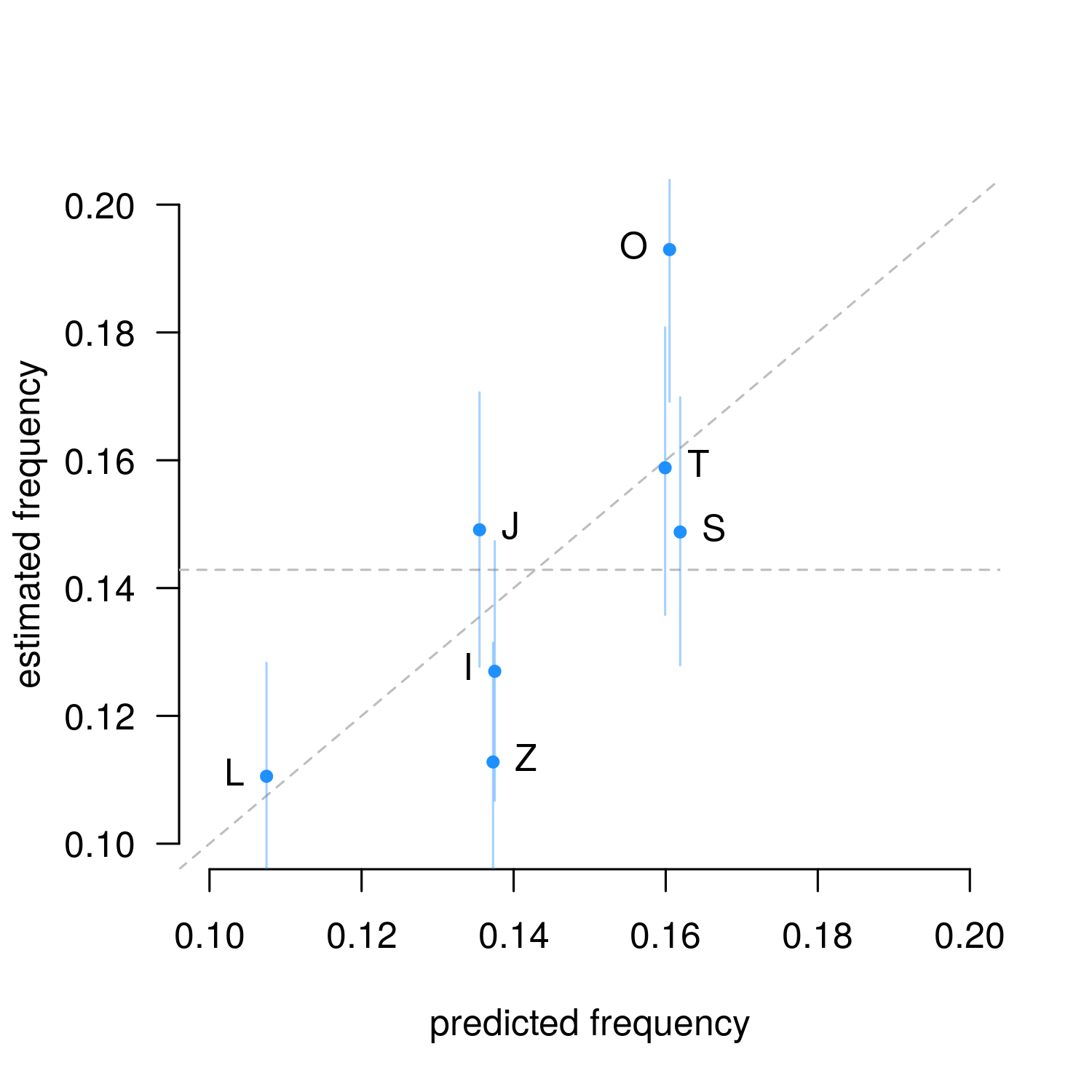Figure 1. Categorical parameter estimates from Gameboy data (n = 692, means and 89% HPDI). The slanted line indicates observations match predictions, the horizontal line indicates uniform random sampling.

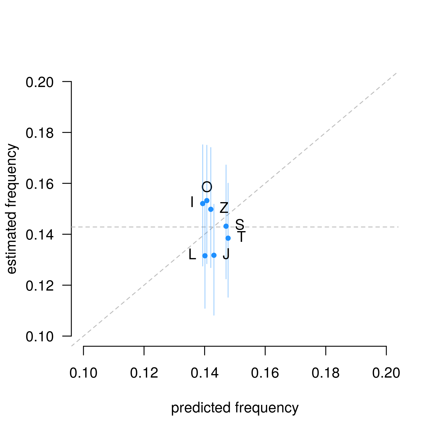
Figure 2. Categorical parameter estimates from NES data (n = 579, means and 89% HPDI). The slanted line indicates observations match predictions, the horizontal line indicates uniform random sampling.

As we expected, the Gameboy algorithm is hard on Z, and favors S, T and especially O, which appears in 19% of actual draws. But this isn’t really good evidence that either algorithm is accurate, since most estimates are not distinct from the horizontal line-of-evenness at 1/7th. Only the L-piece in the Gameboy is a clear match with the simulation. The other estimates could have come from the algorithm, but they could be from something else too. We need to go deeper…

Fitting the Markov models

To estimate proper Markov models, and maybe get clearer results, we adapt the Stan model above to see the past states in the chain.

data {
  int<lower = 1> K; // number of unique outcomes (here, 7)
  int<lower = 1> T; // length of the chain
  int<lower = 1, upper = K> y[T]; // Markov chain data
  vector<lower = 0>[K] theta_prior[K]; // prior on transitions
}
parameters {
  simplex[K] theta[K]; // transition probabilities
}
model {
  for (k in 1:K){
    theta[k] ~ dirichlet(theta_prior[k]);
  }
  for (t in 2:T) y[t] ~ categorical(theta[y[t - 1]]);
}

Our theta changes from a vector holding seven probabilities into seven vectors, one for each state we could be in at time t - 1. This is the transition matrix, now with 49 parameters instead of 7. We give each vector in theta its own Dirichlet prior as before, and update the model using the stan function in R.² The estimates of each of the 49 posterior estimates is comparable to the 49 frequencies from the limiting distribution of the Markov chain:

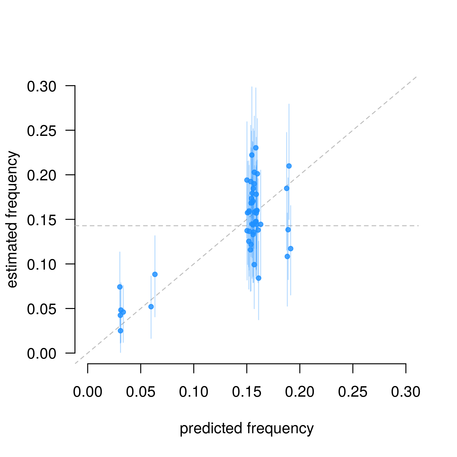
Figure 3. Markov parameter estimates from NES data (n = 579, means and 89% HPDI). The slanted line indicates observations match predictions, the horizontal line indicates uniform random sampling.

As predicted, the real data shows a strong bias against two-in-a-row outcomes (the bottom left estimates). This is strong evidence that the NES algorithm we wrote is an accurate reflection of what we see in the ‘real world’ of gameplay on the NES, e.g. at the Classic Tetris World Championships.

To prepare the Markov model for the Gameboy data, we must allow it to see the last two draws as follows:

data {
  int<lower = 1> K; // number of unique outcomes (here, 7)
  int<lower = 1> T; // length of the chain
  int<lower = 1, upper = K> y[T]; // markovian data vector
  simplex[K] theta_prior[K, K]; // prior on transitions
}
parameters {
  simplex[K] theta[K, K]; // transition probabilities
}
model {
  for (k in 1:K){
    for(j in 1:K){
      theta[k][j] ~ dirichlet(theta_prior[k][j]);
    }
  }
  for (t in 3:T) y[t] ~ categorical(theta[y[t - 2]][y[t - 1]]);
}

The theta object now has another dimension - rather than 7 vectors, we now need 7 $\times$ 7 vectors for 49 states in the system. We can pass the data into this model as above, giving estimates for all 343 parameters to compare against the predicted values:

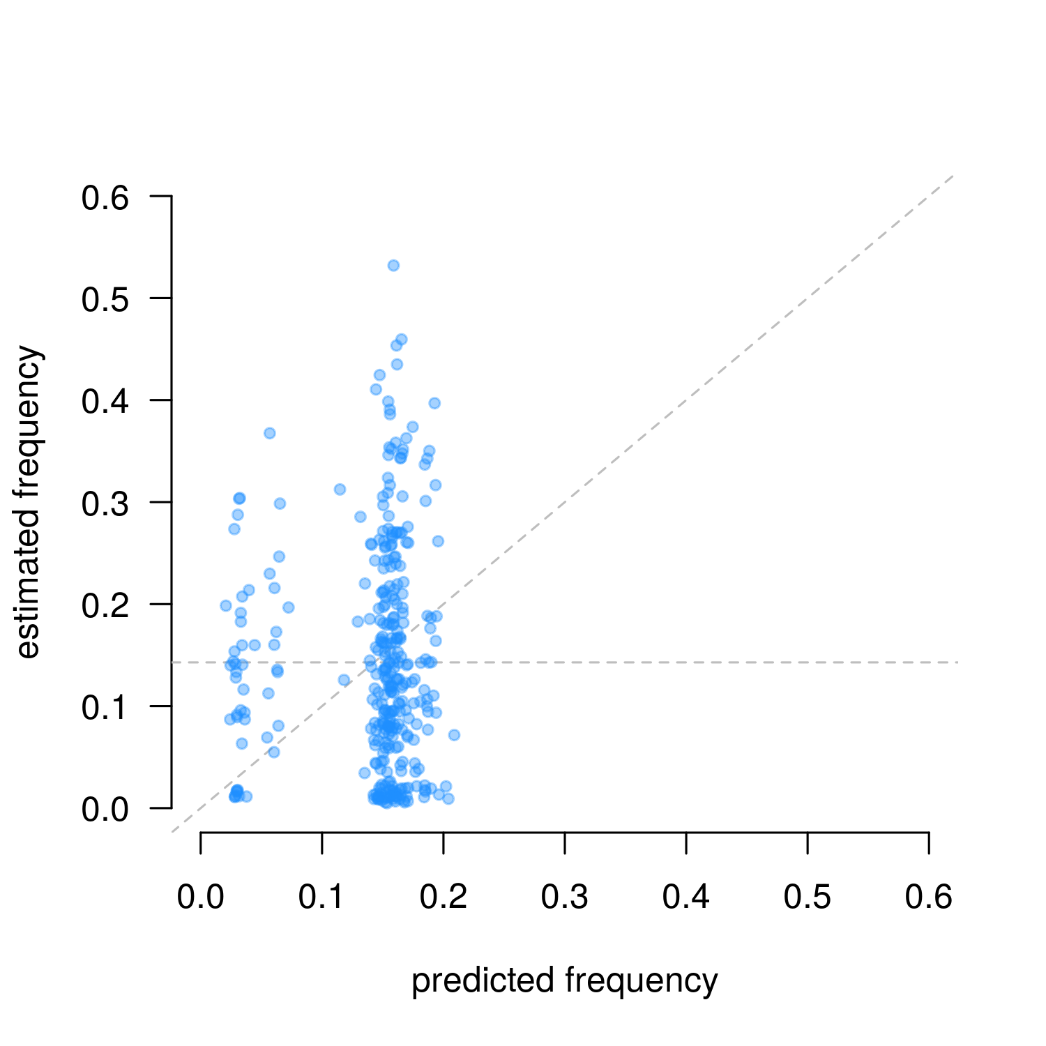
Figure 4. Second-order Markov parameter estimates from Gameboy data (n = 692, means only). The slanted line indicates observations match predictions, the horizontal line indicates uniform random sampling.

Compared to the NES results, this is not very satisfying. With 343 parameters and only 692 data points, some effects were accurately predicted, but others are totally unclear, or clearly inaccurate. We still do not know if the simulation really matches real data.

What to do? One solution is just to collect more data, which would bring our estimates into sharper focus. But more data takes time and energy to prepare (which I have been told is not in the family budget). There is a simpler way, though.

Measuring Signals of Bias

Our simulation of the Gameboy’s transition matrix shows a number of symmetries we can use. In 12 of the 49 Markov states, each one starting with an O, S or T, three outcomes of the seven are substantially favored with a 27% chance each, or, a +38% bias towards picking a ‘favorite’ piece³. This simple yes-or-no event is a signal of the Gameboy’s unique behavior and we only need a simple Binomial model with one parameter to describe it (rather than the monstrous, 343-parameter, second-order Markov model above).

Specifically, if the chain visits one of those 12 special states $n$ times, and in those visits a “favorite” outcome is picked $x$ times, then we’ll say $x$ follows a Binomial distribution with parameters $n$ and $\gamma$,

$$ X \sim \mathrm{Binomial}(n, p) $$ $$ p = 3/7 + \gamma $$

We write it this way, so that the $\gamma$ parameter is the signal of bias - it is exactly 0 with random sampling, but about 0.348 in the Gameboy algorithm. If we set a Beta prior on $p$, we don’t even need to use Stan - the Beta-Binomial conjugacy means that the posterior distribution on the Binomial probability is also Beta distributed,

$$ p \sim \mathrm{Beta}(x + a, (n - x) + b) $$

where $a$ and $b$ define a prior for what $p$ could be (with three favored outcomes of seven, let’s say $a$ = 3 and $b$ = 4). This means we can find the mean and variance of the bias signal as:

p_mean <- (x + 3) / (n + 7) # prior on p is Beta(3, 4)
gamma_mean <- p_mean - 3/7
gamma_sd <- sqrt(p_mean * (1 - p_mean) / (n + 7 + 1))

In the real Gameboy data we collected, the chain visits these twelve special states $n$ = 188 times, and a “favorite” piece was chosen $x$ = 156 times. Updating our signal model with this data, we find $\gamma$ = 0.387($\pm$ 0.028), in almost exact agreement with the predictions from the simulation!⁴

Model symmetries let us test our predictions with only 692 observations, but we didn’t even need this much data. If we plot the expected $x$ for any $n$ under each hypothesis, and compare to the observed data in each chain, the two algorithms quickly diverge:

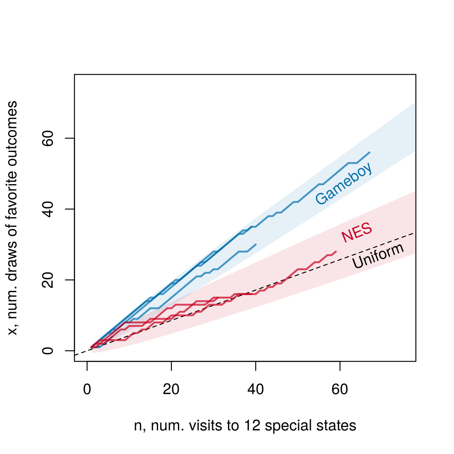
Figure 5. Counts of $x$ and $n$ for each round of Tetris played, the 95% confidence intervals each algorithm, and the expected value under Uniform sampling.

After only about 120 draws (so an special-state $n$ between 30 and 40), the behavior of the two algorithms is clearly different, and we know which is which.

Conclusions

From the above, it looks like the Tetris randomizer algorithms we tried are right. The NES algorithm, with its 49 parameters, was pretty easy to test using the multistate Markov model. But when real data is expensive to collect, or the model becomes too complex, it’s better to forgo the full model and instead find special signals - like our parameter $\gamma$ - to test our predictions.

all data and code for this project is available here